Assignment 3
这次作业需要我们实现蒙特卡洛采样和环境光遮蔽
搜解决办法的时候发现,关于随机数,pbrt的2D Sampling with Multidimensional Transformations讲得挺清楚的…
首先需要实现将均匀分布转换成各种随机分布的函数
Part 1
src/warp.cpp里有所有我们需要实现的函数定义
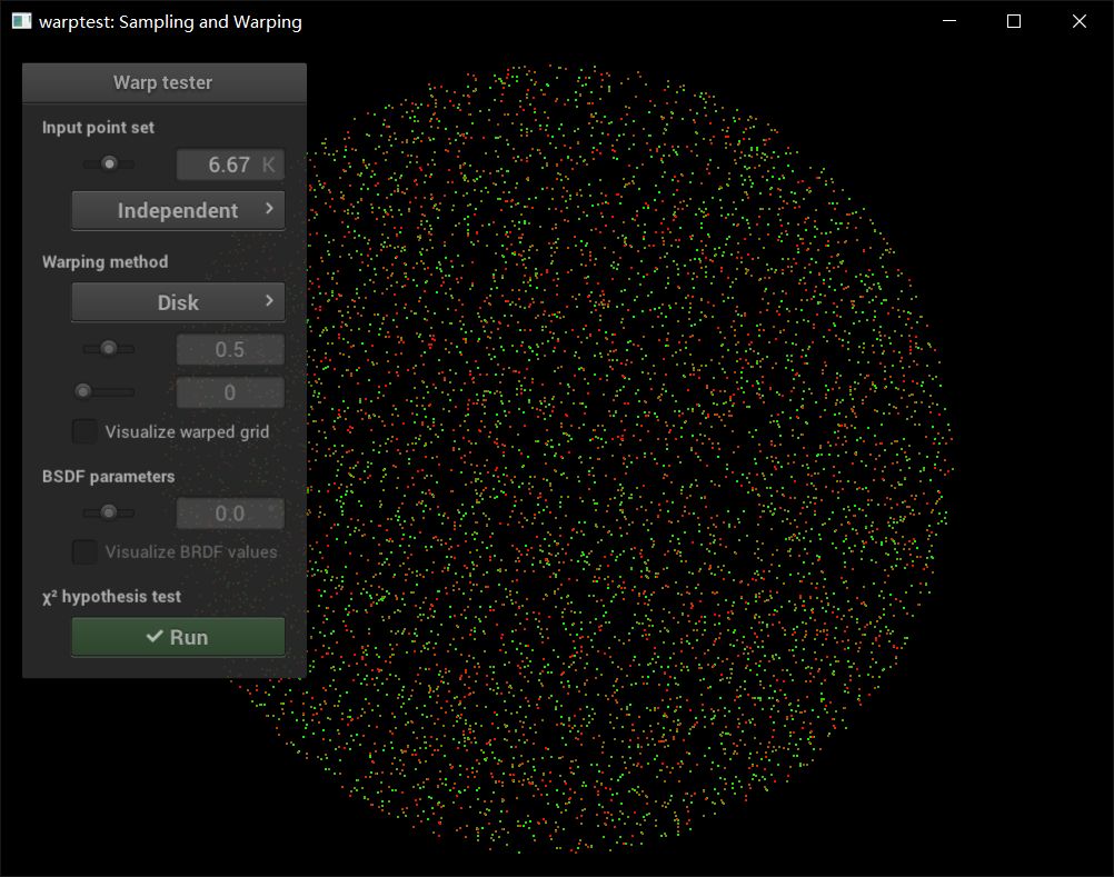
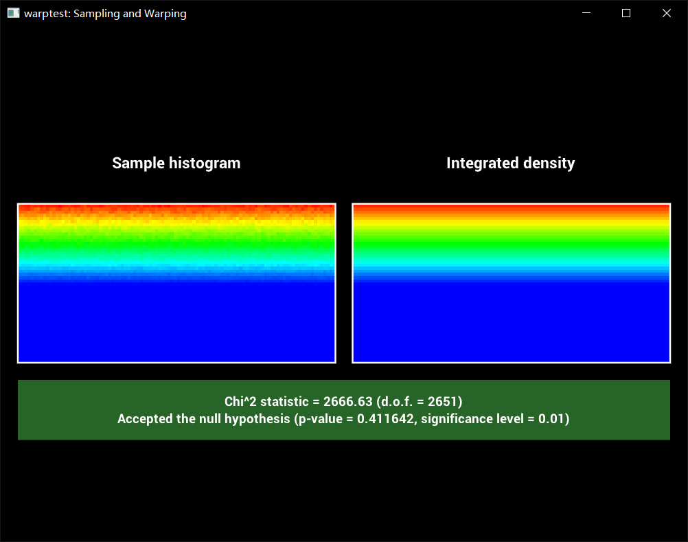
nori提供了一个可视化程序来验证公式的正确性,编译运行warptest就可以看到生成的随机数
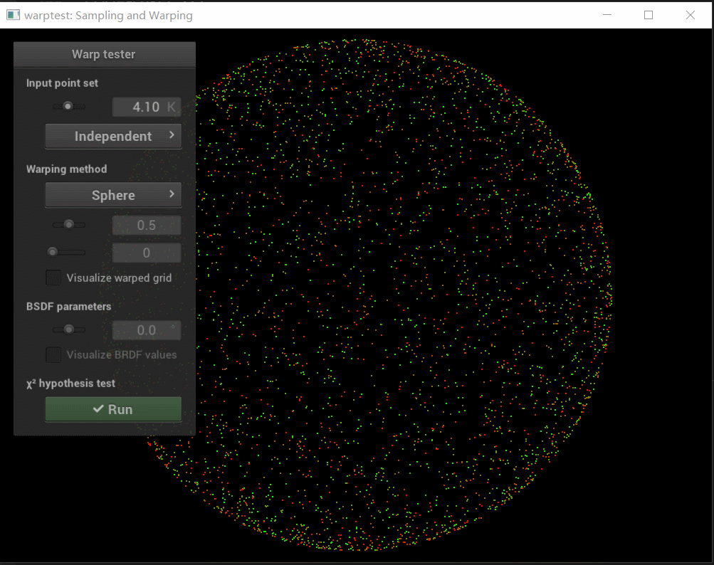
直接启动试试
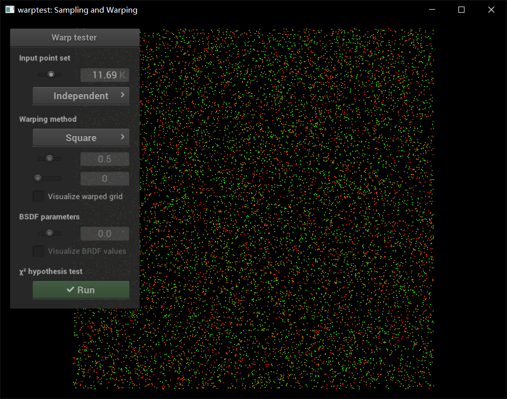
均匀分布,挺好看的
之前Release模式编译启动,程序直接闪退,用Debug启动发现某个地方非法访问…github页面的readme说这版本nano gui有bug…我换了那课程github组织页面最新的就没问题了
将单位矩形上均匀分布的坐标转化为其他分布的方法是:
- 根据概率密度函数计算概率分布函数
- 求概率分布函数的反函数
- 根据上一步求出的函数,将坐标映射到新坐标
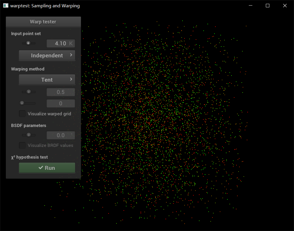
Tent
帐篷?
概率密度函数长这样
p(x,y)=p1(x)p1(y)andp1(t)=⎩⎨⎧1−∣t∣,0,−1≤t≤1otherwise
积分一下,求分布函数
P1(t)=⎩⎨⎧0,21(t+1)2,21(t−1)2,1,t<−1−1≤t<00≤t≤11<t
求一下反函数
P1−1(t)=⎩⎨⎧2t−1,1−2−2t,0≤t<2121≤t<1
可以直接把反函数和概率密度写成代码了
1
2
3
4
5
6
7
8
9
10
11
12
| float tent(float x) {
return x < 0.5f ? sqrt(2.0f * x) - 1.0f : 1.0f - sqrt(2.0f - 2.0f * x);
}
Point2f Warp::squareToTent(const Point2f& sample) {
return Point2f(tent(sample.x()), tent(sample.y()));
}
float tentPdf(float t) {
return t >= -1 && t <= 1 ? 1 - abs(t) : 0;
}
float Warp::squareToTentPdf(const Point2f& p) {
return tentPdf(p.x()) * tentPdf(p.y());
}
|
编译运行
将单位矩形内的点映射到单位圆盘上
有两个随机变量可以用,可以一个用来表示旋转角度,一个用来表示半径,这样是极坐标系,再转换回直角坐标系
极坐标系和直角坐标系转化:
⎩⎨⎧x=rcosθy=rsinθ
概率密度就是点到圆心距离是不是超过1,是的话密度为0,不是的话密度是圆面积分之1
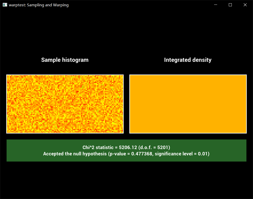
直接写成代码,启动!
1
2
3
4
5
6
7
8
| Point2f Warp::squareToUniformDisk(const Point2f& sample) {
float radius = sample.x();
float angle = sample.y() * (float)M_PI * 2;
return Point2f(radius * cos(angle), radius * sin(angle));
}
float Warp::squareToUniformDiskPdf(const Point2f& p) {
return std::sqrt(p.x() * p.x() + p.y() * p.y() <= 1.0f) ? INV_PI : 0.0f;
}
|
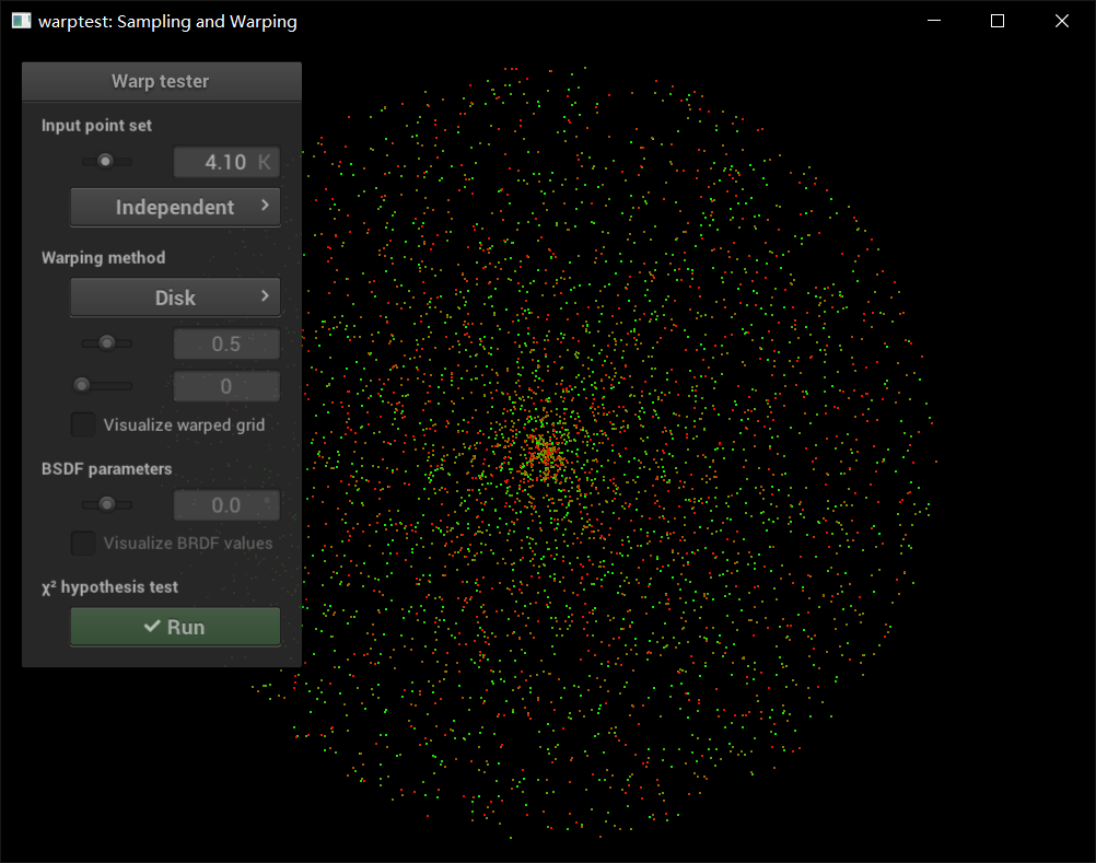
emm这明显是错的…
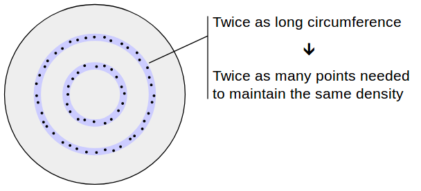
实际上,随着半径增长,圆的周长增长是线性的,因此,可能落在这一圈圆上的点的数量也是线性增长,也就是说,概率密度函数是
f(x)=2x
0到1范围积分一下,概率分布函数是
F(x)=x2
反函数是
F(y)=x
所以均匀分布映射到半径要加个根号
修正代码
1
2
3
4
5
| Point2f Warp::squareToUniformDisk(const Point2f& sample) {
float radius = std::sqrt(sample.x());
float angle = sample.y() * (float)M_PI * 2;
return Point2f(radius * cos(angle), radius * sin(angle));
}
|
运行
说实话,理论我还没完全懂,放个链接球谐光照与PRT学习笔记(二):蒙特卡洛积分与球面上的均匀采样
将单位矩形内的点映射到单位球面上
和圆盘一样,可以使用球坐标系
⎩⎨⎧x=rsinθcosφy=rsinθsinφz=rcosθ
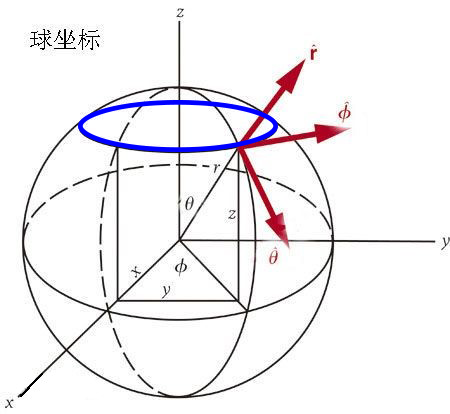
和圆盘一模一样,只有仰角不是均匀的,随着仰角增加,仰角所在那一圈圆的周长(就图里蓝色那一圈)的变化就是概率密度
f(x)=2sin(x)
概率分布函数
F(x)=2−cos(x)+1
反函数
F(y)=acos(1−2x)
球表面积是4π,所以概率密度就是4π1
可以直接写出代码
1
2
3
4
5
6
7
8
9
10
11
12
| Vector3f Warp::squareToUniformSphere(const Point2f& sample) {
float phi = sample.x() * M_PI * 2;
float theta = acos(1 - 2 * sample.y());
float sinTheta = sin(theta);
float cosTheta = cos(theta);
float sinPhi = sin(phi);
float cosPhi = cos(phi);
return Vector3f(sinTheta * cosPhi, sinTheta * sinPhi, cosTheta);
}
float Warp::squareToUniformSpherePdf(const Vector3f& v) {
return INV_FOURPI;
}
|
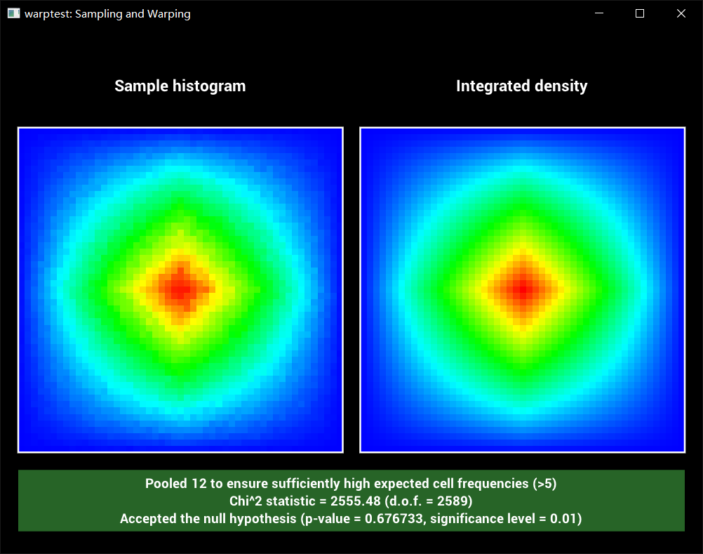
测试一下
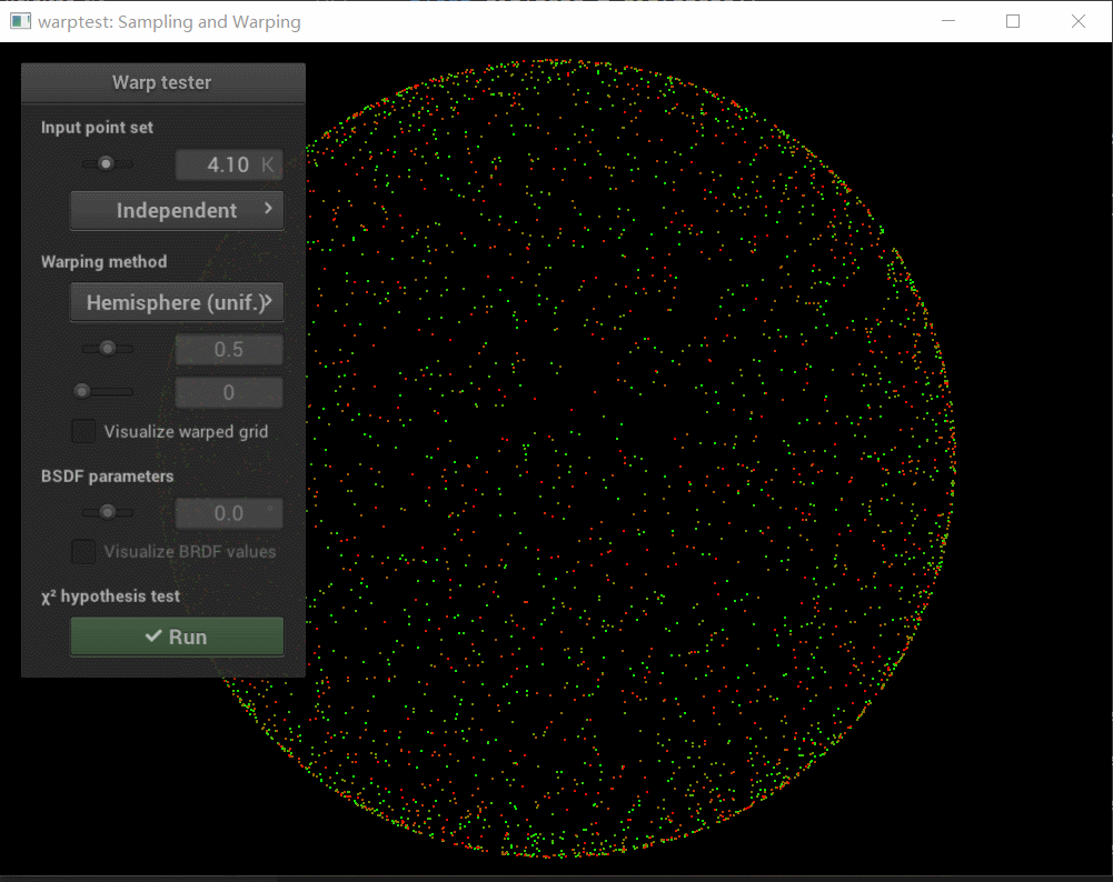
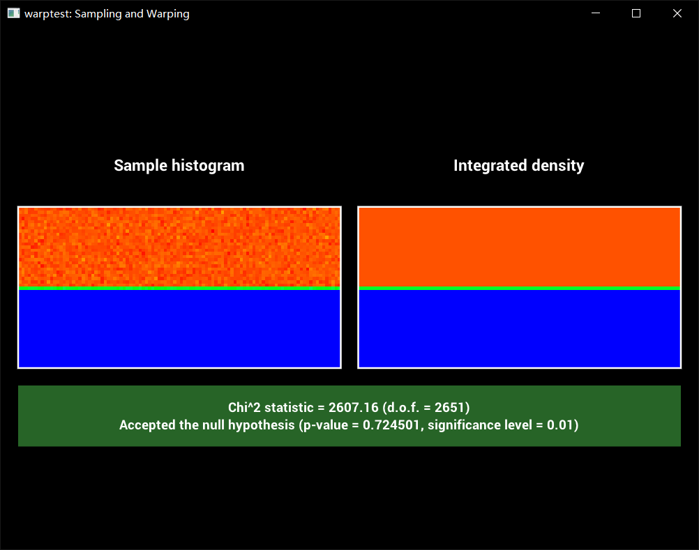
将单位矩形内的点映射到单位半球面上,方向是(0,0,1)
和上面球基本一样,只是因为是半球,所以仰角取值缩小到[0,2π]
直接写代码
1
2
3
4
5
6
7
8
9
10
11
12
| Vector3f Warp::squareToUniformHemisphere(const Point2f& sample) {
float phi = sample.x() * M_PI * 2;
float theta = acos(1 - sample.y());
float sinTheta = sin(theta);
float cosTheta = cos(theta);
float sinPhi = sin(phi);
float cosPhi = cos(phi);
return Vector3f(sinTheta * cosPhi, sinTheta * sinPhi, cosTheta);
}
float Warp::squareToUniformHemispherePdf(const Vector3f& v) {
return v.z() < 0 ? 0 : INV_TWOPI;
}
|
测试一下
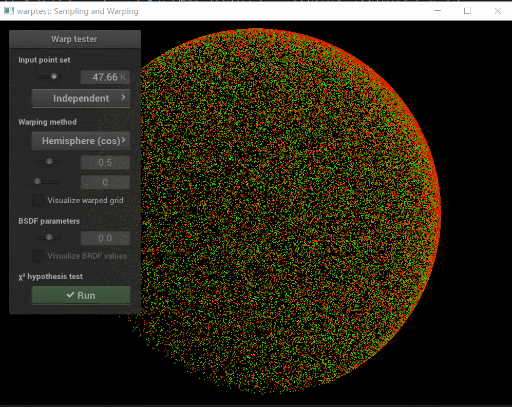
Cosine Hemisphere
将单位矩形内的点映射到单位半球面上,使用余弦密度函数
p(θ)=πcosθ
根据pbrt里说的,把均匀圆盘映射到半球面上就完事了
(具体严格证明还看不懂…)
1
2
3
4
5
6
7
8
9
| Vector3f Warp::squareToCosineHemisphere(const Point2f& sample) {
Point2f bottom = squareToUniformDisk(sample);
float x = bottom.x();
float y = bottom.y();
return Vector3f(x, y, sqrt(1 - x * x - y * y));
}
float Warp::squareToCosineHemispherePdf(const Vector3f& v) {
return v.z() < 0 ? 0 : v.z() * INV_PI;
}
|
Beckmann
将单位矩形内的点映射到Beckmann分布
???这tm完全搞不懂了
D(θ,ϕ)=2π1⋅α2cos3θ2eα2−tan2θ
概率密度直接给出来了饿
1
2
3
4
5
6
7
8
9
10
11
12
13
14
15
16
17
18
19
20
21
22
23
24
| Vector3f Warp::squareToBeckmann(const Point2f& sample, float alpha) {
float phi = M_PI * 2 * sample.x();
float theta = atan(sqrt(-alpha * alpha * log(1 - sample.y())));
float cosPhi = cos(phi);
float sinPhi = sin(phi);
float cosTheta = cos(theta);
float sinTheta = sin(theta);
float x = sinTheta * cosPhi;
float y = sinTheta * sinPhi;
float z = cosTheta;
return Vector3f(x, y, z);
}
float Warp::squareToBeckmannPdf(const Vector3f& m, float alpha) {
if (m.z() <= 0) {
return 0;
}
float alpha2 = alpha * alpha;
float cosTheta = m.z();
float tanTheta2 = (m.x() * m.x() + m.y() * m.y()) / (cosTheta * cosTheta);
float cosTheta3 = cosTheta * cosTheta * cosTheta;
float azimuthal = INV_PI;
float longitudinal = exp(-tanTheta2 / alpha2) / (alpha2 * cosTheta3);
return azimuthal * longitudinal;
}
|
Part 2
第二部分终于进入光照着色部分了
Point Light
需要实现点光源直接光采样,公式已经给出来了
L(x)=4π2Φ∥x−p∥2max(0,cosθ)V(x↔p)
其中,可见性项V,如果着色点和光源之间有物体遮挡,就设为0,否则为1
V(x↔p):={1,0,if x and p are mutually visibleotherwise
照着公式写就完事了,没什么难的
1
2
3
4
5
6
7
8
9
10
11
12
13
14
15
16
17
18
19
| Color3f Li(const Scene* scene, Sampler* sampler, const Ray3f& ray) const {
Intersection its;
if (!scene->rayIntersect(ray, its)) {
return Color3f(0.0f);
}
const auto& frame = its.shFrame;
Point3f x = its.p;
Point3f p = m_lightPos;
auto wo = p - x;
auto woDir = wo.normalized();
float visiblity = 1;
if (scene->rayIntersect(Ray3f(x + wo * 0.00001f, wo))) {
visiblity = 0;
}
auto cosTheta = frame.cosTheta(frame.toLocal(woDir));
auto s = std::pow((x - p).norm(), 2.0f);
auto li = (m_lightEnergy / (4 * M_PI * M_PI)) * ((std::max(0.0f, cosTheta)) / s) * visiblity;
return li;
}
|
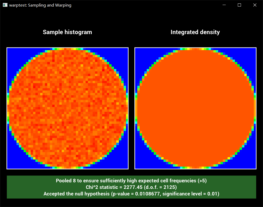
启动!然后程序华丽的挂掉了…debug挂上,发现是可见性检查时的相交测试出现数组索引越界…
检查了一下我们Accel::rayIntersect函数,发现当shadowRay无论是不是true我们都会去计算之后的重心坐标
将shadowRay为true时直接返回true,不去计算后续就完事了
再次启动!
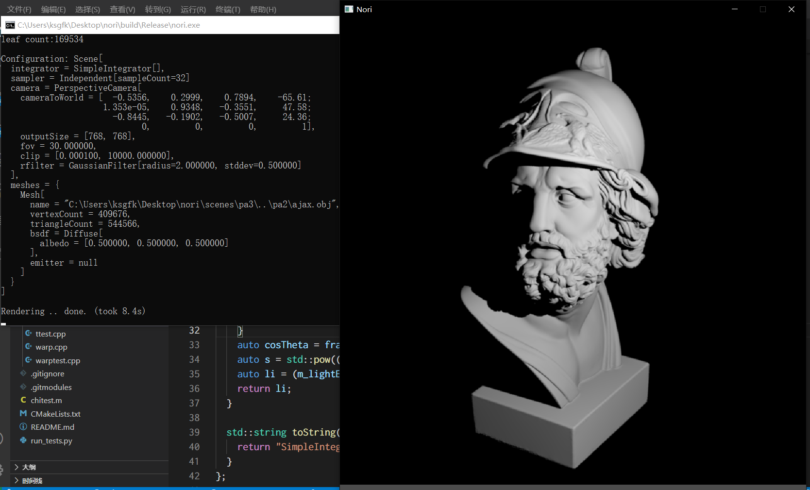
芜湖,起飞
Ambient Occlusion
需要实现环境光遮蔽的效果,它假设物体表面接收从各个方向来的均匀的光,可见性是最重要的。环境光遮蔽的计算公式是:
L(x)=∫H2(x)V(x,x+αωi)πcosθdωi
这个公式是定义在以x点为中心的一个半球上的积分,θ是入射方向和表面在x点法线的夹角,变量α调整遮蔽程度
我们需要半球上余弦权重来采样出射方向,就是使用Part1部分我们实现的Warp::squareToCosineHemisphere函数
可以写出代码:
这里想要使用Sampler类里的函数需要include nori/sampler.h,要使用squareToCosineHemisphere需要include nori/warp.h
1
2
3
4
5
6
7
8
9
10
11
12
13
14
15
16
| Color3f Li(const Scene* scene, Sampler* sampler, const Ray3f& ray) const {
Intersection its;
if (!scene->rayIntersect(ray, its)) {
return Color3f(0.0f);
}
const auto& frame = its.shFrame;
auto rng = sampler->next2D();
auto h = Warp::squareToCosineHemisphere(rng);
auto p = frame.toWorld(h);
auto pN = p.normalized();
int visiblity = 0;
if (!scene->rayIntersect(Ray3f(its.p + pN * 0.00001f, pN))) {
visiblity = 1;
}
return Color3f(float(visiblity));
}
|
启动!
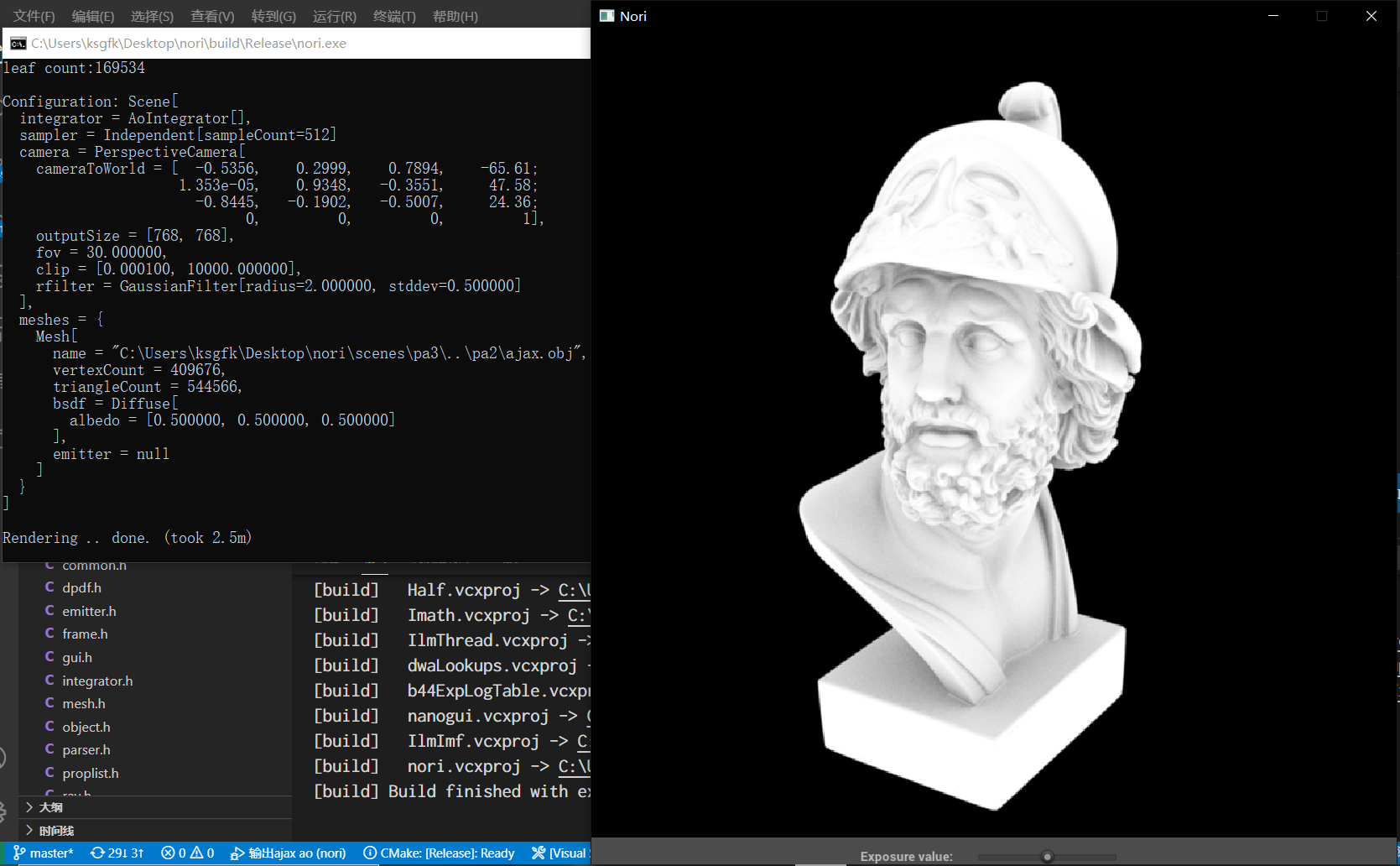
有点慢了…看了下场景文件,采样512次…怪不得…